IBM Quantum Challenge 2020 - Part 3

Dec 9, 2020 14 min read

This post is part of a serie of posts on my experience with the IBM Quantum Challenge 2020.

The serie is organised as follow:

Introduction to the problem.
Mathematical reformulation of the problem.
Unoptimised implementation of the solution (this post).
How to optimise a quantum circuit?.
Optimising multi-controlled X gates.
Optimising the QRAM (Quantum Random Access Memory).

This post will follow a step-by-step approach to guide you on the path of implementing a quantum algorithm to solve the 3^rd problem of the IBM Quantum Challenge.

Overall algorithm

Before digging into the implementation details and problem-specific algorithms, lets discuss a little bit about the main algorithm we will be using.

The challenge rules are clear: Grover’s algorithm^wiki,
qiskit should be used and only 1 iteration is allowed.

The implementation of Grover’s algorithm with 1 iteration is shown in the following quantum circuit.

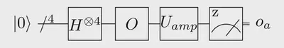
Circuit for Grover's algorithm with 1 iteration. Ancillary qubits are ignored for the moment. $O$ is the oracle, i.e. a quantum circuit that flips the phase of the quantum state only when it encodes the index of the unsolvable board. $U\_{amp}$ is the amplification operator of Grover's algorithm. — Circuit for Grover’s algorithm with 1 iteration. Ancillary qubits are ignored for the moment. $O$ is the oracle, i.e. a quantum circuit that flips the phase of the quantum state only when it encodes the index of the unsolvable board. $U_{amp}$ is the amplification operator of Grover’s algorithm.

We can already implement most of the quantum gates represented:

from qiskit import QuantumCircuit, QuantumRegister

def mcz(register_size: int) -> QuantumCircuit:
    """Returns a multi-controlled Z gate."""
    assert register_size > 1, (
        "Cannot apply a multi-controlled Z without any control."
    )
    qr = QuantumRegister(register_size)
    circuit = QuantumCircuit(qr)
    circuit.h(qr[-1])
    circuit.mcx(qr[:-1], qr[-1])
    circuit.h(qr[-1])
    return circuit

def U_amp(qubit_numbers: int) -> QuantumCircuit:
    """Apply the amplification step of Grover's algorithm."""
    mcz_gate = mcz(qubit_numbers)

    q = QuantumRegister(qubit_numbers)
    circuit = QuantumCircuit(q)
    circuit.h(q)
    circuit.x(q)
    circuit.append(mcz_gate, q)
    circuit.x(q)
    circuit.h(q)
    return circuit

The only quantum gate that is non-trivial to implement is the oracle $O$.

Implementation of the oracle

The oracle $O$ is only defined by its behaviour: it should flip (i.e. multiply by -1) the phase of the quantum state that represents the index of the only non-solvable board.

To do so, the oracle will need to perform 3 steps:

Load the classical data on the quantum computer. This step is needed because we are forbiden to pre-process the boards with a classical computer, meaning that the quantum computer should do all the job and have access to the boards.
Recognise the only board that is not solvable and flip its phase.
Uncompute the classical data loading to avoid ending up with an highly entangled state.

As we will see later, step 3 is not strictly needed to have a correct solution. Nevertheless, this is a common step in quantum computing and removing it felt like cheating, so we will keep this step for the moment.

Step 3 is trivial once step 1 is done as it suffice to reverse the quantum circuit obtained for step 1 to implement step 3. As such, I will only speak about steps 1 and 2 in the following sections.

Step 1 – Data loading using a QRAM

We are trying to load the 16 boards provided by IBM mentors into our quantum registers. The first question that should be answered is “how do we encode a board?”.

Mapping boards to qubits

Two encodings finished in the short-list:

Encode the asteroids on 7 qubits in a superposition state \[\sum_{i = 0}^{5} \vert i \rangle \vert c_{i}\rangle \vert r_i \rangle\] where $i$ is the asteroid index, $c_i$ its column index and $r_i$ its row index.
Encode each cell of the board on 1 qubit and set this qubit to $\vert 1 \rangle$ if and only if an asteroid is on this cell, for a total of 16 qubits.

The first encoding does not use a lot of qubits but has the downsides of being less trivial to use and of not using fully the superposition on its first 3 qubits as we already know there will only be 6 asteroids (for 8 possibilities on 3 qubits).

On the other side, the second encoding is probably the most simple we could think of, with the downside of requiring 16 over the 28 available.

After careful thinking, I chose the second encoding for several reasons:

The number of used qubits does not impact the cost that will used to evaluate the final circuit but the number of gates does. In this sense, the second encoding is better.
The implementation of the 2 steps described above was easy to devise for the second encoding, which seemed to not be the case for the first one.

Now that the encoding is clear, how do we actually load one board on our quantum register?

Encoding one board

Let take the unsolvable board of IBM mentor’s dataset as an example.

The only unsolvable board from IBM mentor's dataset. — The only unsolvable board from IBM mentor’s dataset.

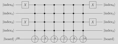
We use a row-major order to encode our board and want to end up with the state $$\vert 0100\ 0001\ 1100\ 1010 \rangle$$ if and only if the qubits encoding the board index was in the state $\vert 1010\rangle$ (binary writing of the decimal number “10”).

Note that the quantum state encoding the board is shown in big endian meaning that the left-most bit is the bit at index $15$ and the right-most bit has the index $0$.

Once formulated the problem is actually quite simple to solve: we just have to execute a bunch of controlled-$X$ gates as shown in the following quantum circuit.

Quantum circuit encoding the only unsolvable board (index 10 i.e. $\vert 1010 \rangle$) of IBM mentor's dataset. Indices added in the crosses denote the target qubit of the multi-controlled $X$ gate. — Quantum circuit encoding the only unsolvable board (index 10 i.e. $\vert 1010 \rangle$) of IBM mentor’s dataset. Indices added in the crosses denote the target qubit of the multi-controlled $X$ gate.

The corresponding code is

import typing as ty
from qiskit import QuantumCircuit, QuantumRegister

BoardEncoding = ty.List[ty.Tuple[str, str]]

def encode_problem(
        problem: BoardEncoding, problem_index: int
) -> QuantumCircuit:
    """
    Encode the given problem on the qboard register if the
    qindex register matches the given problem_index.

    This function returns a quantum circuit that encodes the given problem
    on the |qboard> register only if the |qindex> register encodes the
    given problem_index.

    :param problem: a list of asteroid coordinates, given as tuples
        of strings.
    :param problem_index: the index of the board.
    """
    qindex = QuantumRegister(4)
    qboard = QuantumRegister(16)
    circuit = QuantumCircuit(qindex, qboard)

    bin_index = bin(problem_index)[2:].zfill(4)

    for i, bit_value in enumerate(bin_index):
        if bit_value == "0":
            circuit.x(qindex[i])

    for x, y in problem:
        cell_index = 4 * int(x) + int(y)
        circuit.mcx(qindex, qboard[cell_index])

    # Uncompute.
    # We do not have to reverse the order here because all the
    # gates can be executed in parallel.
    for i, bit_value in enumerate(bin_index):
        if bit_value == "0":
            circuit.x(qindex[i])

    return circuit

Some of you might realise that the circuit implemented above is quite simple to optimise. You are right and it will be optimised in the next blog post.

Encoding all the boards

Once we know how to encode one board it becomes trivial to encode all the boards: just repeat the one board encoding procedure for each board.

def qram(problem_set: ty.List[BoardEncoding]):
    """
    Encodes the given problem set into the |qboard> register.

    The returned routine takes as inputs:
    - |qindex> that encodes the indices for which we want to encode the
      boards. The |qindex> register will likely be given in a
      superposition of all the possible states.
    - |qboard> that should be given in the |0> state and that is returned
      in the state that encodes the problem_set given. For each qindex,
      the |qboard> state in |qindex>|qboard> is full of |0> except on the
      locations where there is an asteroid, in which case the state is |1>.
    """
    qindex = QuantumRegister(4)
    qboard = QuantumRegister(16)
    circuit = QuantumCircuit(qindex, qboard)

    for problem_index, problem in enumerate(problem_set):
        circuit.append(
            encode_problem(problem, problem_index),
            # List of all the qubits we apply the problem encoding
            # procedure to.
            [*qindex, *qboard],
        )
    return circuit

If you are unfamiliar with the “star-notation” used you can have a look at this stackoverflow answer.

Step 2 – Phase flipping

Now that our QRAM is implemented, the only missing piece is the procedure that will flip the phase of a non-solvable board.

We saw in the last post that any non-solvable board “includes” a permutation matrix.

There are $4! = 24$ permutation matrices of size $4\times 4$ which means that checking all the possibilities is doable for such a small size.

The number of permutation matrices of size $n\times n$ is $n!$, which is HUGE. The algorithm described here is fine for a $4\times 4$ board but would be super-uber costly for a $10\times 10$ board ($10! = 3628800$ possible permutation matrices).

An algorithm with a better complexity exists but at the time being I was in a rush to have a working solution and did not investigate further, knowing that my algorithm was fine for a $4\times 4$ board but would completely blow up for bigger sizes.

My algorithm was simple: enumerate all the $24$ possible permutations and check for each of them if the board “includes” this permutation.

Repetition of the only unsolvable board from IBM mentor's dataset. The 24 possible permutations are highlighted in orange (or blue in dark-mode). If at least one of the board has 4 asteroids highlighted then it is impossible to solve it with only 3 shots. — Repetition of the only unsolvable board from IBM mentor’s dataset. The 24 possible permutations are highlighted in orange (or blue in dark-mode). If at least one of the board has 4 asteroids highlighted then it is impossible to solve it with only 3 shots.

The algorithm is: for each permutation, use a 4-controlled $X$ gate where the 4 control qubits are qubits in the $\vert \mathrm{qboard} \rangle$ register and whose indices are given by the current permutation.

To take an example, checking for the identity (which is one of the 24 permutations) is simply applying a 4-controlled $X$ gate with $\left\{ \vert \mathrm{qboard}_i \rangle \right\}_{i \in \{ 0, 5, 10, 15 \}}$ as control registers and an ancilla qubit as target.

def check_if_match_permutation(permutation: ty.List[int]) -> QuantumCircuit:
    """
    Construct a quantum circuit to check if the given qboard state
    "includes" the given permutation.

    The |qancilla> qubit is flipped if |qboard> includes the given
    permutation.
    """
    qboard = QuantumRegister(16)
    qancilla = QuantumRegister(1)
    circuit = QuantumCircuit(qboard, qancilla)

    qubit_indices = [
        4 * row + col for row, col in enumerate(permutation)
    ]
    circuit.mcx([qboard[i] for i in qubit_indices], qancilla)

    return circuit

Still, there is one issue with that approach. What about boards that “include” more than one permutation?

Example of a single board that includes 2 different permutations.

Such a board will not be marked as “non-solvable” by the current algorithm. The reason is simple: the ancilla qubit flipped when a permutation is spotted in the board would be flipped twice.

The solution to this issue? An adder of course. But before explaining we should note a little property.

A $4 \times 4$ board with 6 asteroids cannot include more than two $4 \times 4$ permutations matrices.

This is due to the fact that 2 different permutation matrices differ in at least 2 rows and 2 columns.

The proof by contradiction is quite straightforward: imagine that we have a board with 6 asteroids that includes 3 permutation matrices or more. The first permutation matrix overlaps with 4 asteroids. The second permutation matrix overlaps with at least 2 other asteroids (from the property above). The third and last permutation matrix should overlap with at least 2 other asteroids (not already overlapped by the first or second permutation matrices), but this is impossible because this would require at least 8 asteroids on the board.

So in the worst case we have a board that includes 2 permutation matrices. This means that we can count the number of permutation matrices that are included in a given board on 2 qubits, with the help of an adder.

def get_2_qubit_adder_gate():
    """
    Returns a quantum circuit implementing an adder.

    The adder adds a 1-qubit value to a 2-bit register without
    any overflow check.
    """
    a = QuantumRegister(1)
    b = QuantumRegister(2)
    circuit = QuantumCircuit(a, b)

    circuit.ccx(a, b[0], b[1])
    circuit.cx(a, b[0])

    return circuit

To summarise the algorithm is:

Count the number of permutations that are included in the given board.
Flip the phase if the counter is non-zero.
Undo the first step.

I implemented this with the following code:

from itertools import permutations

def check_if_match_any_permutation():
    """
    Flip the phase of the boards that include at least 1 permutation.

    This quantum circuit takes a board on 16 qubits and flip the phase
    of the quantum state if the board includes at least 1 permutation.
    """
    qboard = QuantumRegister(16)
    qadded = QuantumRegister(1)
    qcounter = QuantumRegister(2)
    circuit = QuantumCircuit(qboard, qadded, qcounter)

    add_gate = get_2_qubit_adder_gate()
    all_permutations = list(permutations(range(4), 4))

    for perm in all_permutations:
        checker = check_if_match_permutation(perm)
        circuit.append(checker, [*qboard, *qadded])
        circuit.append(add_gate, [*qadded, *qcounter])
        circuit.append(checker.inverse(), [*qboard, *qadded])

    circuit.z(qcounter)

    for perm in reversed(all_permutations):
        checker = check_if_match_permutation(perm)
        circuit.append(checker.inverse(), [*qboard, *qadded])
        circuit.append(add_gate.inverse(), [*qadded, *qcounter])
        circuit.append(checker, [*qboard, *qadded])

    return circuit

We can simplify the phase-flip procedure to a simple $Z$ gate on the two qubits of the counter because we know that the only possible non-zero numbers of permutations included in a given board are 1 ($\vert 01 \rangle$) and 2 ($\vert 10 \rangle$). The risk of flipping the phase twice is excluded because a board cannot include 3 ($\vert 11 \rangle$) permutations.

Glue the pieces together

The only task left to have a working solution is to write down the code that will glue together the QRAM, the oracle and will implement 1 iteration of Grover’s algorithm.

from qiskit import ClassicalRegister

def grover_oracle_week3(problem_set) -> QuantumCircuit:
    """
    Flip the phase of the only index representing a non-solvable board.

    This oracle needs a total of 23 qubits:
    - 4 qubits for the |index> register
    - 16 qubits for the |board> register, that should be given in the
      |0> state.
    - 3 ancilla qubits.
    """
    qindex = QuantumRegister(4)
    qboard = QuantumRegister(16)
    qancilla = QuantumRegister(3)
    circuit = QuantumCircuit(qindex, qboard, qancilla)

    qram_gate = qram(problem_set)
    checker = check_if_match_any_permutation()

    circuit.append(qram_gate, [*qindex, *qboard,])
    circuit.append(checker, [*qboard, *qancilla])
    circuit.append(qram_gate.inverse(), [*qindex, *qboard])

    return circuit


def week3_ans_func(problem_set) -> QuantumCircuit:
    """
    Returns a quantum circuit solving the given problem.
    """
    qindex = QuantumRegister(4)
    qboard = QuantumRegister(16)
    qancilla = QuantumRegister(3)
    cindex = ClassicalRegister(4)
    circuit = QuantumCircuit(qindex, qboard, qancilla, cindex)

    oracle = grover_oracle_week3(problem_set)
    diffusion = U_amp(4)

    circuit.h(qindex)

    # Perform only 1 iteration to stick to the rules.
    for _ in range(1):
        circuit.append(oracle, [*qindex, *qboard, *qancilla])
        circuit.append(diffusion, qindex)

    circuit.measure(qindex, cindex)
    circuit = circuit.reverse_bits()
    return circuit

We are now ready to compute the cost of our code and run it to check if it outputs the correct answer.

Analysis of the generated circuit

The whole code is available in this Gist.

Checking the circuit validity

The first thing to do once you think your implementation is finished is to check it. Fortunately IBM mentors gave us a test set, so we can simulate the quantum circuit on our local machine.

The following code execute a 23-qubit quantum circuit on your machine. While your memory should be fine, your CPU might spike at 100% (or more) for several seconds.

from qiskit import Aer, execute

problem_set = [
    [["0", "2"], ["1", "0"], ["1", "2"], ["1", "3"], ["2", "0"], ["3", "3"]],
    [["0", "0"], ["0", "1"], ["1", "2"], ["2", "2"], ["3", "0"], ["3", "3"]],
    [["0", "0"], ["1", "1"], ["1", "3"], ["2", "0"], ["3", "2"], ["3", "3"]],
    [["0", "0"], ["0", "1"], ["1", "1"], ["1", "3"], ["3", "2"], ["3", "3"]],
    [["0", "2"], ["1", "0"], ["1", "3"], ["2", "0"], ["3", "2"], ["3", "3"]],
    [["1", "1"], ["1", "2"], ["2", "0"], ["2", "1"], ["3", "1"], ["3", "3"]],
    [["0", "2"], ["0", "3"], ["1", "2"], ["2", "0"], ["2", "1"], ["3", "3"]],
    [["0", "0"], ["0", "3"], ["1", "2"], ["2", "2"], ["2", "3"], ["3", "0"]],
    [["0", "3"], ["1", "1"], ["1", "2"], ["2", "0"], ["2", "1"], ["3", "3"]],
    [["0", "0"], ["0", "1"], ["1", "3"], ["2", "1"], ["2", "3"], ["3", "0"]],
    [["0", "1"], ["0", "3"], ["1", "2"], ["1", "3"], ["2", "0"], ["3", "2"]],
    [["0", "0"], ["1", "3"], ["2", "0"], ["2", "1"], ["2", "3"], ["3", "1"]],
    [["0", "1"], ["0", "2"], ["1", "0"], ["1", "2"], ["2", "2"], ["2", "3"]],
    [["0", "3"], ["1", "0"], ["1", "3"], ["2", "1"], ["2", "2"], ["3", "0"]],
    [["0", "2"], ["0", "3"], ["1", "2"], ["2", "3"], ["3", "0"], ["3", "1"]],
    [["0", "1"], ["1", "0"], ["1", "2"], ["2", "2"], ["3", "0"], ["3", "1"]],
]

circuit = week3_ans_func(problem_set)

backend_sim = Aer.get_backend("qasm_simulator")
job = execute(circuit, backend_sim, shots=8192)
result = job.result()
counts = result.get_counts()

print(counts)

The output of executing the quantum circuit is

{
  '0000': 281,
  '0001': 268,
  '0010': 302,
  '0011': 310,
  '0100': 284,
  '0101': 283,
  '0110': 265,
  '0111': 298,
  '1000': 273,
  '1001': 283,
  '1010': 3922,
  '1011': 258,
  '1100': 303,
  '1101': 286,
  '1110': 292,
  '1111': 284
}

which shows that we measured the result $\vert 1010\rangle$ is by far the most frequent. And $1010$ is exactly 10, i.e. the index of the only non-solvable board!

If you simulate the quantum circuit on your laptop you will likely have different results. The counts displayed above have been obtained by sampling the computed quantum state and as such they may differ slightly from one execution to another.

The only important point here is that the result $\vert 1010 \rangle$ appears significantly more frequently than the other states.

Cost

The goal of the challenge is to produce the quantum circuit with the lowest possible cost to solve the given problem, the cost of a quantum circuit being defined as

from qiskit.transpiler import PassManager
from qiskit.transpiler.passes import Unroller

def cost(circuit: QuantumCircuit) -> int:
    """Compute the cost of a circuit"""
    pass_ = Unroller(["u3", "cx"])
    pm_unroll = PassManager(pass_)
    unrolled_circuit = pm_unroll.run(circuit)
    ops = unrolled_circuit.count_ops()
    return 10 * ops.get("cx", 0) + ops.get("u3", 0)

With this definition we can compute the cost of our quantum circuit:

print(f"Cost of the generated quantum circuit: {cost(circuit)}")

which should compute a cost of 144 423.

Conclusion

In this post I explained how I implemented my first solution to the third IBM Quantum Challenge exercise.

The implementation explained in this post was aiming at validity, i.e. having an implementation that effectively solve the problem. In the next blog post, we will refine and optimise this implementation to target efficiency, i.e. reducing the cost of our implementation as much as possible.

Click if you want to know my final score

In the next posts I will explain how I lowered down my score from 144 423 to 9 258.